ATOMIC
STRUCTURE
Information collected from
http://chemed.chem.purdue.edu/genchem/topicreview/
http://wine1.sb.fsu.edu/chm1045/notes/Atoms/AtomStr1/
http://www.chemistry.ohio-state.edu/~grandinetti/teaching/Chem121/lectures/
http://library.thinkquest.org/19662/low/eng/exp-rutherford.html
http://library.thinkquest.org/19662/low/eng/model-bohr.html?tqskip1=1
http://www.chemtopics.com/lectures/unit04/lecture1/l1u4.htm
http://www-theory.chem.washington.edu/~trstedl/quantum/quantum.html
http://science.howstuffworks.com/atom5.htm
Fundamental subatomic particles
|
Particle |
Symbol |
Charge |
Mass |
|
electron |
e- |
-1 |
0.0005486 amu |
|
proton |
p+ |
+1 |
1.007276 amu |
|
neutron |
no |
0 |
1.008665 amu |
The first evidence for sub-atomic particles came
from experiments with the conduction of electricity through gases in sealed
glass tubes at low pressures. In
the late 19th century, chemists and physicists were studying the relationship
between electricity and matter. They were placing high voltage electric
currents through glass tubes filled with low-pressure gas (mercury, neon,
xenon) much like neon
lights. Electric current was carried from one electrode (cathode)
through the gas to the other electrode (anode) by a beam called cathode
rays.

In 1897, a British physicist, J. J. Thomson did
a series of experiments with the following results:
- He
found that if the tube was placed within an electric or magnetic field,
then the cathode rays could be deflected or moved (this is how the the
cathode ray tube (CRT) on your television
works).
- By applying an
electric field alone, a magnetic field alone, or both in combination, Thomson could measure the ratio of the
electric charge to the mass of the cathode rays.
- He found the same
charge to mass ratio of cathode rays was seen regardless of what material
was inside the tube or what the cathode was made of.
Thomson concluded the following:
- Cathode
rays were made of tiny, negatively charged particles,
which he called electrons.
- The electrons
had to come from inside the atoms of the gas or metal electrode.
- Because the
charge to mass ratio was the same for any substance, the electrons were
a basic part of all atoms.
- Because the
charge to mass ratio of the electron was very high, the electron must
be very small.
Later, an American Physicist named Robert Milikan measured the electrical charge of an electron. With
these two numbers (charge, charge to mass ratio), physicists calculated the
mass of the electron as 9.10 x 10⁻²⁸ grams. For comparison, a U.S.
penny has a mass of 2.5 grams; so, 2.7 x 1027 or 2.7 billion billion billion electrons would
weigh as much as a penny!
Two other conclusions came from the
discovery of the electron:
- Because the
electron was negatively charged and atoms are electrically neutral, there
must be a positive charge somewhere in the atom.
- Because
electrons are so much smaller than atoms, there must be other, more
massive particles in the atom.
From these results, Thomson proposed a model of the atom that was like a
watermelon. The red part was the positive charge and the seeds were the
electrons. In 1909 Robert Millikan used the
classic oil drop experiment to determine the charge on these particles.
J.J. Thomson demonstrated in 1897 that the
rays consist of a stream of negatively charged particles which he called electrons. He was able to measure the charge/mass
ratio of these particles and found this to be the same regardless of what gas
was in the tube or what metal the electrodes were made from.
Using the smallest charge obtained and Thomson's
charge/mass ratio the electron mass is roughly 1/2000 the mass of the lightest
atom. Thus there are obviously particles smaller than atoms.
Thomson's dilemma:
how could matter containing electrons be neutral and where was all the mass?
Other experiments with discharge tubes suggested the
existence of a positive particle with much greater mass (the proton).
- Goldstein
discovered canal rays (Kanalstrahlen) in 1886
- Wien and Thomson saw positive rays moving in
opposite direction of cathode rays.
- Properties of
protons:
charge, same as electron but positive
mass 1.67262314e-27 kg, mass of H less the electron mass
spin ½
magnetic moment, 2.7928474 nuclear magnetic moment
Based on this evidence Thomson proposed the first atomic model with
sub-atomic particles.
Neutrons (Chadwick (1932) discovered neutron-neutral charge particles in the
nucleus)
- Bothe, Becker,
Joliot, Curie and Chadwick observed some very penetrating particles when
they bombarded beryllium with alpha particles.
- The reaction is now
known as
Be + a = C + n + Energy
- James Chadwick
(1891-1974) discovered and confirmed neutrons from the reaction
B + n = Li + a + Energy
Rutherford´s model of the atom
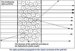 In the years
1909-1911 Ernest Rutherford
and his students - Hans Geiger (1882-1945) and Ernest Marsden
conducted some experiments to search the problem of alpha particles scattering
by the thin gold-leaf.
In the years
1909-1911 Ernest Rutherford
and his students - Hans Geiger (1882-1945) and Ernest Marsden
conducted some experiments to search the problem of alpha particles scattering
by the thin gold-leaf.
Radioactivity
Wilhelm Roentgen (1895) discovered that when cathode
rays struck certain materials (copper for example) a different type of ray was
emitted. This new type of ray, called the "x" ray had the following
properties:
- The could pass
unimpeded through many objects
- They were
unaffected by magnetic or electric fields
- They produced
an image on photographic plates (i.e. they interacted with silver
emulsions like visible light)
Henri Becquerel (1896) was studying materials which
would emit light after being exposed to sunlight (i.e. phosphorescent
materials). The discovery by Roentgen made Becquerel wonder if the
phosphorescent materials might also emit x- rays. He discovered that uranium
containing minerals produced x-ray radiation (i.e. high energy photons).
Marie and Pierre Curie set about to isolate the
radioactive components in the uranium mineral.
Ernest Rutherford studied alpha rays, beta rays and
gamma rays, emitted by certain radioactive substances. He noticed that each
behaved differently in response to an electric field:
- The b-rays were attracted to
the anode
- The a-rays were attracted to
the cathode
- The g-rays were not affected
by the electric field
The a and b "rays"
were composed of (charged) particles and the g-"ray" was high energy radiation (photons)
similar to x-rays
- b-particles are high speed
electrons (charge = -1)
- a-particles are the
positively charged core of the helium atom (charge = +2)
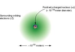
- Most of the
mass of the atom, and all its positive charge, reside in a very small
dense centrally located region called the "nucleus"
- Most of the
total volume of the atom is empty space within which the negatively
charged electrons move around the nucleus

Chadwick (1932) discovers neutron - neutral charge
particles in the nucleus
The number of protons, neutrons, and electrons in an
atom can be determined from a set of simple rules.
 The number of protons
in the nucleus of the atom is equal to the atomic number (Z).
The number of protons
in the nucleus of the atom is equal to the atomic number (Z). - The number of
electrons in a neutral atom is equal to the number of protons.
- The mass
number of the atom (M) is equal to the sum of the number of protons
and neutrons in the nucleus.
- The number of
neutrons is equal to the difference between the mass number of the atom (M)
and the atomic number (Z).
We use the following symbol to describe the atom:
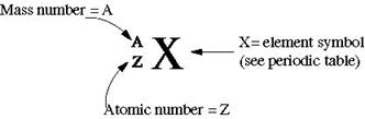
A= Z + N, where N is the number of neutrons.
If you add or subtract a proton from the
nucleus, you create a new element.
If you add or subtract a neutron from the
nucleus, you create a new isotope of the same element you started with.
 In a neutral atom, the number of positively charged
protons in the nucleus is equal to the number of orbiting electrons.
In a neutral atom, the number of positively charged
protons in the nucleus is equal to the number of orbiting electrons.
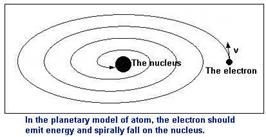
But, the model created by Rutherford had still some
serious discordance. According to the classic science, electron moving around
the nucleus should emit an electromagnetic wave. That kind of emission is
connected with the escape of some energy from the electron-ion circuit.
Electron should than move not by the circle but helical and finally collide
with the nucleus. But atom is stable. Other discordance regarded the radiation
- it were to be constant (because the time of electron's cycle in accordance
with the lost of energy should change constantly) and spectral lines shouldn't
occur.
The model of atom created by Rutherford couldn't be the
conclusive model of matter's constitution.
Electromagnetic Theory of Radiation
Much of what is known about the structure of the
electrons in an atom has been obtained by studying the interaction between
matter and different forms of electromagnetic radiation. Electromagnetic
radiation has some of the properties of both a particle and a wave.
Particles have a definite mass and they occupy space. Waves
have no mass and yet they carry energy as they travel through space. In
addition to their ability to carry energy, waves have four other characteristic
properties: speed, frequency, wavelength, and amplitude. The frequency (v)
is the number of waves (or cycles) per unit of time. The frequency of a wave is
reported in units of cycles per second (s-1) or hertz (Hz).
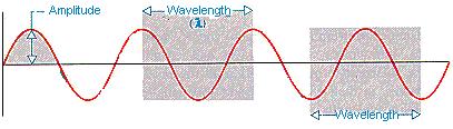
The idealized drawing of a wave in the figure below
illustrates the definitions of amplitude and wavelength. The wavelength
(l) is the smallest distance between repeating points on the wave. The amplitude
of the wave is the distance between the highest (or lowest) point on the wave
and the center of gravity of the wave.
If we measure the frequency (v) of a wave in
cycles per second and the wavelength (l) in meters, the product of these
two numbers has the units of meters per second. The product of the frequency (v)
times the wavelength (l) of a wave is therefore the
speed (s) at which the wave travels through space. l l = s
Light and Other Forms of Electromagnetic
Radiation
Light is a wave with both electric and magnetic
components. It is therefore a form of electromagnetic radiation.
Visible light contains the narrow band of frequencies
and wavelengths in the portion of the electro-magnetic spectrum that our eyes
can detect. It includes radiation with wavelengths between about 400 nm
(violet) and 700 nm (red). Because it is a wave, light is bent when it enters a
glass prism. When white light is focused on a prism, the light rays of
different wavelengths are bent by differing amounts and the light is
transformed into a spectrum of colors. Starting from
the side of the spectrum where the light is bent by the smallest angle, the colors are red, orange, yellow, green, blue, and violet.
As we can see from the following diagram, the energy carried
by light increases as we go from red to blue across the visible spectrum.
Because the wavelength of electromagnetic radiation
can be as long as 40 m or as short as 10-5 nm, the visible spectrum
is only a small portion of the total range of electromagnetic radiation.
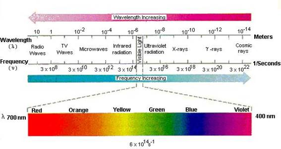
The electromagnetic spectrum includes radio and TV
waves, microwaves, infrared, visible light, ultraviolet, x-rays, g-rays, and
cosmic rays, as shown in the figure above. These different forms of radiation
all travel at the speed of light (c). They differ, however, in their
frequencies and wavelengths. The product of the frequency times the wavelength
of electromagnetic radiation is always equal to the speed of light. vl = c
As a result, electromagnetic
radiation that has a long wavelength has a low frequency, and radiation with a
high frequency has a short wavelength.
When an electric current is passed through a glass
tube that contains hydrogen gas at low pressure the tube gives off blue light.
When this light is passed through a prism (as shown in the figure below), four
narrow bands of bright light are observed against a
black background.
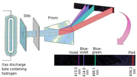
These narrow bands have the characteristic wavelengths
and colors shown in the table below.
|
Wavelength |
|
|
Color |
|
|
|
656.2 |
|
|
red |
|
|
|
486.1 |
|
|
blue-green |
|
|
|
434.0 |
|
|
blue-violet |
|
|
|
410.1 |
|
|
violet |
|
|
Four more series of lines were discovered in the emission
spectrum of hydrogen by searching the infrared spectrum at longer wave-lengths
and the ultraviolet spectrum at shorter wavelengths. Each of these lines fits
the same general equation, where n1 and n2
are integers and RH is 1.09678 x 10⁻² nm-1.
The system of the
lines was called the Balmer spectral series. For hydrogen there are also some other
series:
- The Lyman spectral series - placed in ultraviolet - is described by the
first formula (given above) but n' is equal 1 here, and n is equal 2 or
bigger.
- The Pachen spectral
series - placed in
infra-red - is described by the first formula but n' is equal 3 here, and
n is equal 4 or bigger.
- The Brackett spectral series - placed in infra-red - is described by the
first formula but n' is equal 4 here, and n is equal 5 or bigger.
The spectral lines of the other elements which are heavier than hydrogen are
more complicated.
Explanation of the Emission Spectrum
Max Planck presented a theoretical explanation of the
spectrum of radiation emitted by an object that glows when heated. He argued
that the walls of a glowing solid could be imagined to contain a series of
resonators that oscillated at different frequencies. These resonators gain
energy in the form of heat from the walls of the object and lose energy in the
form of electromagnetic radiation. The energy of these resonators at any moment
is proportional to the frequency with which they oscillate.
To fit the observed spectrum, Planck had to assume
that the energy of these oscillators could take on only a limited number of
values. In other words, the spectrum of energies for these oscillators was no
longer continuous. Because the number of values of the energy of these
oscillators is limited, they are theoretically "countable." The
energy of the oscillators in this system is therefore said to be quantized.
Planck introduced the notion of quantization to explain how light was emitted.
Albert Einstein extended Planck's work to the light
that had been emitted. At a time when everyone agreed that light was a wave
(and therefore continuous), Einstein suggested that it behaved as if it was a
stream of small bundles, or packets, of energy. In other words, light was also
quantized. Einstein's model was based on two assumptions. First, he assumed
that light was composed of photons, which are small, discrete bundles of
energy. Second, he assumed that the energy of a photon is proportional to its frequency. E
= hv
In this equation, h is a constant known as
Planck's constant, which is equal to 6.626 x 10⁻³⁴ J-s.
Example: Let's calculate the energy of a single photon
of red light with a wavelength of 700.0 nm and the energy of a mole of these photons.
Red light with a wavelength of 700.0 nm has a
frequency of 4.283 x 10¹⁴ s-1.
Substituting this frequency into the Planck-Einstein equation gives the
following result.
![]()
A single photon of red light carries an insignificant
amount of energy. But a mole of these photons carries about 171,000 joules of
energy, or 171 kJ/mol.
![]()
Absorption of a mole of photons of red light would
therefore provide enough energy to raise the temperature of a liter of water by more than 40oC.
The fact that hydrogen atoms emit or absorb radiation
at a limited number of frequencies implies that these atoms can only absorb
radiation with certain energies. This suggests that there are only a limited
number of energy levels within the hydrogen atom. These energy levels are
countable. The energy levels of the hydrogen atom are quantized.
Niels Bohr proposed a
model for the hydrogen atom that explained the spectrum of the hydrogen atom.
The Bohr model was based on the following assumptions.
- The electron
in a hydrogen atom travels around the nucleus in a circular orbit.
- The energy of
the electron in an orbit is proportional to its distance from the nucleus.
The further the electron is from the nucleus, the more energy it has.
- Only a limited
number of orbits with certain energies are allowed. In other words, the orbits are quantized.
- The only
orbits that are allowed are those for which the angular momentum of the
electron is an integral multiple of Planck's constant divided by 2p.
- Light is
absorbed when an electron jumps to a higher energy orbit and emitted when
an electron falls into a lower energy orbit.
- The energy of
the light emitted or absorbed is exactly equal to the difference between
the energies of the orbits.
Some of the key elements of this hypothesis are
illustrated in the figure below.
Three points deserve particular attention. First, Bohr
recognized that his first assumption violates the principles of classical
mechanics. But he knew that it was impossible to explain the spectrum of the
hydrogen atom within the limits of classical physics. He was therefore willing
to assume that one or more of the principles from classical physics might not
be valid on the atomic scale.
Second, he assumed there are only a limited number of
orbits in which the electron can reside. He based this assumption on the fact
that there are only a limited number of lines in the spectrum of the hydrogen
atom and his belief that these lines were the result of light being emitted or
absorbed as an electron moved from one orbit to another in the atom.
Finally, Bohr restricted the number of orbits on the
hydrogen atom by limiting the allowed values of the angular momentum of the
electron. Any object moving along a straight line has a momentum equal
to the product of its mass (m) times the velocity (v) with which
it moves. An object moving in a circular orbit has an angular momentum
equal to its mass (m) times the velocity (v) times the radius of
the orbit (r). Bohr assumed that the angular momentum of the electron
can take on only certain values, equal to an integer times Planck's constant
divided by 2p.
Bohr then used classical physics to show that the
energy of an electron in any one of these orbits is inversely proportional to
the square of the integer n.
The difference between the energies of any two orbits
is therefore given by the following equation.
In this equation, n1 and n2
are both integers and RH is the proportionality constant
known as the Rydberg constant.
Planck's equation states that the energy of a photon
is proportional to its frequency.
E = hv
Substituting the relationship between the frequency, wavelength,
and the speed of light into this equation suggests that the energy of a photon
is inversely proportional to its wavelength. The inverse of the wavelength of
electromagnetic radiation is therefore directly proportional to the energy of
this radiation.
By properly defining the units of the constant, RH,
Bohr was able to show that the wavelengths of the light given off or absorbed
by a hydrogen atom should be given by the following equation.
Thus, once he introduced his
basic assumptions, Bohr was able to derive an equation that matched the
relationship obtained from the analysis of the spectrum of the hydrogen atom.
At first glance, the Bohr model looks like a
two-dimensional model of the atom because it restricts the motion of the
electron to a circular orbit in a two-dimensional plane. In reality the Bohr
model is a one-dimensional model, because a circle can be defined by specifying
only one dimension: its radius, r. As a result,
only one coordinate (n) is needed to describe the orbits in the Bohr
model.
Unfortunately, electrons aren't particles that can be
restricted to a one-dimensional circular orbit. They act to some extent as
waves and therefore exist in three-dimensional space. The Bohr model works for
one-electron atoms or ions only because certain factors present in more complex
atoms are not present in these atoms or ions. To construct a model that
describes the distribution of electrons in atoms that contain more than one
electron we have to allow the electrons to occupy three-dimensional space. We
therefore need a model that uses three coordinates to describe the distribution
of electrons in these atoms.
Wave-Particle Duality
The theory of wave-particle duality developed
by Louis-Victor de Broglie eventually explained why
the Bohr model was successful with atoms or ions that contained one electron.
It also provided a basis for understanding why this model failed for more
complex systems. Light acts as both a particle and a wave. In many ways light
acts as a wave, with a characteristic frequency, wavelength, and amplitude.
Light carries energy as if it contains discrete photons or packets of energy.
When an object behaves as a particle in motion, it has
an energy proportional to its mass (m) and the
speed with which it moves through space (s).
E = ms2
When it behaves as a wave, however, it has an energy
that is proportional to its frequency:
By simultaneously assuming that an object can be both
a particle and a wave, de Broglie set up the
following equation.

By rearranging this equation, he derived a
relationship between one of the wave-like properties of matter and one of its
properties as a particle.
As noted in the previous section, the product of the
mass of an object times the speed with which it moves is the momentum (p)
of the particle. Thus, the de Broglie equation
suggests that the wavelength (l) of any object in motion is inversely proportional
to its momentum.

De Broglie concluded that
most particles are too heavy to observe their wave properties. When the mass of
an object is very small, however, the wave properties can be detected
experimentally. De Broglie predicted that the mass of
an electron was small enough to exhibit the properties of both particles and
waves. In 1927 this prediction was confirmed when the diffraction of electrons
was observed experimentally by C. J. Davisson.
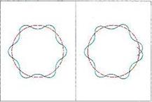 De Broglie applied his theory of wave-particle duality to the
Bohr model to explain why only certain orbits are allowed for the electron. He
argued that only certain orbits allow the electron to satisfy both its particle
and wave properties at the same time because only certain orbits have a
circumference that is an integral multiple of the wavelength of the electron,
as shown in the figure below.
De Broglie applied his theory of wave-particle duality to the
Bohr model to explain why only certain orbits are allowed for the electron. He
argued that only certain orbits allow the electron to satisfy both its particle
and wave properties at the same time because only certain orbits have a
circumference that is an integral multiple of the wavelength of the electron,
as shown in the figure below.
Wave Functions and Orbitals
We still talk about the Bohr model of the atom even if
the only thing this model can do is explain the spectrum of the hydrogen atom
because it was the last model of the atom for which a simple physical picture
can be constructed. It is easy to imagine an atom that consists of solid
electrons revolving around the nucleus in circular orbits.
Erwin Schrödinger combined the equations for the
behaviour of waves with the de Broglie equation to
generate a mathematical model for the distribution of electrons in an atom. The
advantage of this model is that it consists of mathematical equations known as wave
functions that satisfy the requirements placed on the behaviour of
electrons. The disadvantage is that it is difficult to imagine a physical model
of electrons as waves.
The Schrödinger model assumes that the electron is a
wave and tries to describe the regions in space, or orbitals,
where electrons are most likely to be found. Instead of trying to tell us where
the electron is at any time, the Schrödinger model describes the probability
that an electron can be found in a given region of space at a given time. This
model no longer tells us where the electron is; it only tells us where it might
be.
The Heisemberg uncertainty principle
People are familiar with measuring
things in the macroscopic world around them. Someone pulls out a tape measure
and determines the length of a table. A state trooper aims his radar gun at a
car and knows what direction the car is traveling, as
well as how fast. They get the information they want and don't worry whether
the measurement itself has changed what they were measuring. After all, what
would be the sense in determining that a table is 80 cm long if the very act of
measuring it changed its length!
At the atomic scale of quantum
mechanics, however, measurement becomes a very delicate process. Let's say you
want to find out where an electron is and where it is going (that trooper has a
feeling that any electron he catches will be going faster than the local speed
limit). How would you do it? Get a super high powered magnifier and look for
it? The very act of looking depends upon light, which is made of
photons, and these photons could have enough momentum that once they hit the
electron they would change its course! It's like rolling the cue ball across a
billiard table and trying to discover where it is going by bouncing the 8-ball
off of it; by making the measurement with the 8-ball you have certainly altered
the course of the cue ball. You may have discovered where the cue ball was, but
now have no idea of where it is going (because you were measuring with the
8-ball instead of actually looking at the table).
Werner Heisenberg was the first to
realize that certain pairs of measurements have an intrinsic uncertainty
associated with them. For instance, if you have a very good idea of where
something is located, then, to a certain degree, you must have a poor idea of
how fast it is moving or in what direction. We don't notice this in everyday
life because any inherent uncertainty from Heisenberg's principle is well
within the acceptable accuracy we desire. For example, you may see a parked car
and think you know exactly where it is and exactly how fast it is moving. But
would you really know those things exactly? If you were to measure the
position of the car to an accuracy of a billionth of a billionth of a centimeter, you would be trying to measure the positions of
the individual atoms which make up the car, and those atoms would be jiggling
around just because the temperature of the car was above absolute zero!
Heisenberg's uncertainty principle
completely flies in the face of classical physics. After all, the very
foundation of science is the ability to measure things accurately, and now
quantum mechanics is saying that it's impossible to get those measurements
exact! But the Heisenberg uncertainty principle is a fact of nature, and it
would be impossible to build a measuring device which could get around it.
What is the Schrödinger equation?
Every quantum particle is characterized by a wave
function. In 1925 Erwin Schrödinger developed the differential equation which
describes the evolution of those wave functions. By using Schrödinger's
equation scientists can find the wave function which solves a particular
problem in quantum mechanics. Unfortunately, it is usually impossible to find
an exact solution to the equation, so certain assumptions are used in order to
obtain an approximate answer for the particular problem.

Quantum Numbers and Electron configurations
Four numbers used to describe the electrons in an atom.
The Bohr model was a one-dimensional model that
used one quantum number to describe the electrons in the atom. Only the size of
the orbit was important, which was described by the n quantum number. Schrödinger
described an atomic model with electrons in three dimensions. This model
required three coordinates, or three quantum numbers, to describe where
electrons could be found.
The three coordinates from
Schrödinger's wave equations are the principal (n), angular (l),
and magnetic (m) quantum numbers. These quantum numbers describe the
size, shape, and orientation in space of the orbitals
on an atom.
1. Principal (shell) quantum number - n
- Describes the energy level within the atom.
- Energy levels are 1 to 7
- Maximum number of electrons in n is 2 n 2
The principal
quantum number (n) describes the size of the orbital. Orbitals for which n = 2 are larger than those for
which n = 1, for example. Because they have opposite electrical charges,
electrons are attracted to the nucleus of the atom. Energy must therefore be
absorbed to excite an electron from an orbital in which the electron is close
to the nucleus (n = 1) into an orbital in which it is further from the
nucleus (n = 2). The principal quantum number therefore indirectly
describes the energy of an orbital.
2. Momentum (subshell)
quantum number - l
- Describes the sublevel in n
- Sublevels in the atoms of the known elements are
s - p - d - f
- Each energy level has n sublevels.
- Sublevels of different energy levels may have
overlapping energies.
- The momentum quantum number also describes the
shape of the orbital.
- Orbitals have shapes that are best described as
spherical (l = 0), polar (l = 1), or cloverleaf (l =
2).
- Orbitals even take on more complex shapes as the value
of the angular quantum number becomes larger.
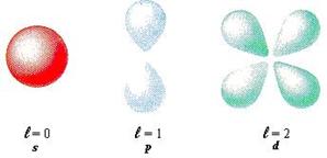
The orbital (angular)
quantum number (l) describes the shape of the orbital. Orbitals have shapes that are best described as spherical (l
= 0), polar (l = 1), or cloverleaf (l = 2). They can even take on
more complex shapes as the value of the angular quantum number becomes larger.
3. Magnetic quantum number - m
- Describes the orbital within a sublevel
- s has 1 orbital
- p has 3 orbitals
- d has 5 orbitals
- f has 7 orbitals
- Orbitals contain 1 or 2 electrons, never more.
- m also describes the direction, or orientation in
space for the orbital.
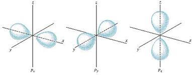
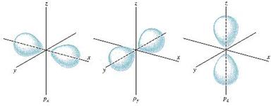
This diagram shows
the three possible orientations of a p orbital - px, py,
pz.
There is only one way in which
a sphere (l = 0) can be oriented in space. Orbitals
that have polar (l = 1) or cloverleaf (l = 2) shapes, however, can
point in different directions. We therefore need a third quantum number, known
as the magnetic quantum number (m), to describe the orientation
in space of a particular orbital. (It is called the magnetic quantum
number because the effect of different orientations of orbitals
was first observed in the presence of a magnetic field.) For example, the p
orbital can line up with the x axis, y axis, or z axis. Numerically, the
options are expressed as –1, 0, and +1. The "middle" orientation is
always expressed as zero, and the others are +/- integers.
4. Spin quantum number - s
- This fourth quantum
number describes the spin of the electron.
- Electrons in the same
orbital must have opposite spins.
- Possible spins are
clockwise or counterclockwise.
To distinguish
between the two electrons in an orbital, we need a fourth quantum number. This
is called the spin quantum number (s) because electrons behave as
if they were spinning in either a clockwise or counterclockwise
fashion. One of the electrons in an orbital is arbitrarily assigned an s
quantum number of +1/2, the other is assigned an s
quantum number of -1/2. Thus, it takes three quantum numbers to define an
orbital but four quantum numbers to identify one of the electrons that can
occupy the orbital.
Rules Governing the Allowed Combinations of
Quantum Numbers
- The three
quantum numbers (n, l, and m) that describe an
orbital are integers: 0, 1, 2, 3, and so on.
- The principal
quantum number (n) cannot be zero. The allowed values of n
are therefore 1, 2, 3, 4, and so on.
- The angular
quantum number (l) can be any integer between 0 and n - 1. If n = 3, for example, l can be either
0, 1, or 2.
- The magnetic quantum number (m) can be any integer between -l
and +l. If l = 2, m can be either
-2, -1, 0, +1, or +2.
Shells and Subshells of Orbitals
Orbitals that have the same
value of the principal quantum number form a shell. Orbitals
within a shell are divided into subshells that
have the same value of the angular quantum number. Chemists describe the shell
and subshell in which an orbital belongs with a
two-character code such as 2p or 4f. The first character
indicates the shell (n = 2 or n = 4). The second character
identifies the subshell. By convention, the following
lowercase letters are used to indicate different subshells.
|
s: |
|
l = 0 |
|
p: |
|
l = 1 |
|
d: |
|
l = 2 |
|
f: |
|
l = 3 |
 Although
there is no pattern in the first four letters (s, p, d, f),
the letters progress alphabetically from that point (g, h, and so
on). Some of the allowed combinations of the n and l quantum
numbers are shown in the figure below.
Although
there is no pattern in the first four letters (s, p, d, f),
the letters progress alphabetically from that point (g, h, and so
on). Some of the allowed combinations of the n and l quantum
numbers are shown in the figure below.
The third rule limiting allowed combinations of the n,
l, and m quantum numbers has an important consequence. It forces
the number of subshells in a shell to be equal to the
principal quantum number for the shell. The n = 3 shell, for example,
contains three subshells: the 3s, 3p,
and 3d orbitals.
Possible Combinations of Quantum
Numbers
There is only one orbital in the n = 1 shell
because there is only one way in which a sphere can be oriented in space. The
only allowed combination of quantum numbers for which n = 1 is the
following.
|
n |
|
l |
|
m |
|
|
|
1 |
|
0 |
|
0 |
|
1s |
There are four orbitals in
the n = 2 shell.
|
n |
|
l |
|
m |
|
|
|
2 |
|
0 |
|
0 |
|
2s |
|
2 |
|
1 |
|
-1 |
|
|
|
2 |
|
1 |
|
0 |
2p |
|
|
2 |
|
1 |
|
1 |
|
There is only one orbital in the 2s subshell. But, there are three orbitals
in the 2p subshell because there are three
directions in which a p orbital can point. One of these orbitals is oriented along the X axis, another along
the Y axis, and the third along the Z axis of a coordinate
system, as shown in the figure below. These orbitals
are therefore known as the 2px, 2py, and 2pz
orbitals.
There are nine orbitals in
the n = 3 shell.
|
n |
|
l |
|
m |
|
|
|
3 |
|
0 |
|
0 |
|
3s |
|
|
|
|
|
|
|
|
|
3 |
|
1 |
|
-1 |
|
|
|
3 |
|
1 |
|
0 |
3p |
|
|
3 |
|
1 |
|
1 |
|
|
|
|
|
|
|
|
|
|
|
3 |
|
2 |
|
-2 |
|
|
|
3 |
|
2 |
|
-1 |
3d |
|
|
3 |
|
2 |
|
0 |
||
|
3 |
|
2 |
|
1 |
||
|
3 |
|
2 |
|
2 |
|
There is one orbital in the 3s subshell and three orbitals in
the 3p subshell. The n = 3 shell,
however, also includes 3d orbitals.
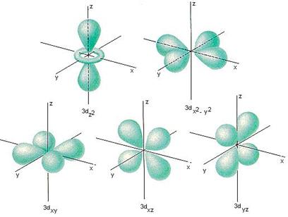
The five different orientations of orbitals
in the 3d subshell are shown in the figure
below. One of these orbitals lies in the XY
plane of an XYZ coordinate system and is called the 3dxy
orbital. The 3dxz and 3dyz orbitals have the same shape, but they lie between the axes
of the coordinate system in the XZ and YZ planes. The fourth
orbital in this subshell lies along the X and Y
axes and is called the 3dx2-y2
orbital. Most of the space occupied by the fifth orbital lies along the Z
axis and this orbital is called the 3dz2 orbital.
The number of orbitals in a
shell is the square of the principal quantum number: 12 = 1, 22
= 4, 32 = 9. There is one orbital in an s
subshell (l = 0), three orbitals
in a p subshell (l = 1), and five orbitals in a d subshell (l
= 2). The number of orbitals in a subshell
is therefore 2(l) + 1.
Before we can use these orbitals
we need to know the number of electrons that can occupy an orbital and how they
can be distinguished from one another. Experimental evidence suggests that an
orbital can hold no more than two electrons.
To distinguish between the two electrons in an
orbital, we need a fourth quantum number. This is called the spin quantum
number (s) because electrons behave as if they were spinning in
either a clockwise or counterclockwise fashion. One
of the electrons in an orbital is arbitrarily assigned an s quantum
number of +1/2, the other is assigned an s
quantum number of -1/2. Thus, it takes three quantum numbers to define an
orbital but four quantum numbers to identify one of the electrons that can
occupy the orbital.
The allowed combinations of n, l, and m
quantum numbers for the first four shells are given in the table below. For
each of these orbitals, there are two allowed values
of the spin quantum number, s.
An applet showing atomic and
molecular orbitals from ![]()
Summary of Allowed Combinations of Quantum
Numbers
|
n |
|
|
l |
|
|
|
m |
Subshell
Notation |
Number of Orbitals in the Subshell |
Number of Electrons Needed
to Fill Subshell |
Total Number of Electrons in
Subshell |
|
|
|||||||||||
|
1 |
|
|
0 |
|
|
|
0 |
1s |
1 |
2 |
2 |
|
|
|||||||||||
|
2 |
|
|
0 |
|
|
|
0 |
2s |
1 |
2 |
|
|
2 |
|
|
1 |
|
|
|
1,0,-1 |
2p |
3 |
6 |
8 |
|
|
|||||||||||
|
3 |
|
|
0 |
|
|
|
0 |
3s |
1 |
2 |
|
|
3 |
|
|
1 |
|
|
|
1,0,-1 |
3p |
3 |
6 |
|
|
3 |
|
|
2 |
|
|
|
2,1,0,-1,-2 |
3d |
5 |
10 |
18 |
|
|
|||||||||||
|
4 |
|
|
0 |
|
|
|
0 |
4s |
1 |
2 |
|
|
4 |
|
|
1 |
|
|
|
1,0,-1 |
4p |
3 |
6 |
|
|
4 |
|
|
2 |
|
|
|
2,1,0,-1,-2 |
4d |
5 |
10 |
|
|
4 |
|
|
3 |
|
|
|
3,2,1,0,-1,-2,-3 |
4f |
7 |
14 |
32 |
The Relative Energies of Atomic Orbitals
 Because of the
force of attraction between objects of opposite charge, the most important factor
influencing the energy of an orbital is its size and therefore the value of the
principal quantum number, n. For an atom that contains only one
electron, there is no difference between the energies of the different subshells within a shell. The 3s, 3p, and 3d
orbitals, for example, have the same energy in a
hydrogen atom. The Bohr model, which specified the energies of orbits in terms
of nothing more than the distance between the electron and the nucleus,
therefore works for this atom.
Because of the
force of attraction between objects of opposite charge, the most important factor
influencing the energy of an orbital is its size and therefore the value of the
principal quantum number, n. For an atom that contains only one
electron, there is no difference between the energies of the different subshells within a shell. The 3s, 3p, and 3d
orbitals, for example, have the same energy in a
hydrogen atom. The Bohr model, which specified the energies of orbits in terms
of nothing more than the distance between the electron and the nucleus,
therefore works for this atom.
The hydrogen atom
is unusual, however. As soon as an atom contains more than one electron, the
different subshells no longer have the same energy.
Within a given shell, the s orbitals always
have the lowest energy. The energy of the subshells
gradually becomes larger as the value of the angular quantum number becomes
larger.
Relative energies: s
< p < d < f
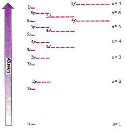
As a result, two
factors control the energy of an orbital for most atoms: the size of the
orbital and its shape, as shown in the figure below.
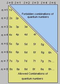
A very simple device can be constructed
to estimate the relative energies of atomic orbitals.
The allowed combinations of the n and l quantum numbers are
organized in a table, as shown in the figure below and arrows are drawn at 45
degree angles pointing toward the bottom left corner of the table.
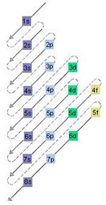 The order of
increasing energy of the orbitals is then read off by
following these arrows, starting at the top of the first line and then
proceeding on to the second, third, fourth lines, and so on. This diagram predicts
the following order of increasing energy for atomic orbitals.
The order of
increasing energy of the orbitals is then read off by
following these arrows, starting at the top of the first line and then
proceeding on to the second, third, fourth lines, and so on. This diagram predicts
the following order of increasing energy for atomic orbitals.
1s < 2s < 2p < 3s
< 3p <4s < 3d <4p < 5s < 4d
< 5p < 6s < 4f < 5d < 6p <
7s < 5f < 6d < 7p < 8s
...
Electron Configurations, the Aufbau Principle, Degenerate Orbitals,
and Hund's Rule
The electron configuration of an atom describes
the orbitals occupied by electrons on the atom. The
basis of this prediction is a rule known as the aufbau
principle, which assumes that electrons are added to an atom, one at a
time, starting with the lowest energy orbital, until all of the electrons have
been placed in an appropriate orbital.
A hydrogen atom (Z = 1) has only one electron,
which goes into the lowest energy orbital, the 1s orbital. This is
indicated by writing a superscript "1" after the symbol for the
orbital.
H (Z = 1): 1s1
The next element has two electrons and the second
electron fills the 1s orbital because there are only two possible values
for the spin quantum number used to distinguish between the electrons in an
orbital.
He (Z = 2): 1s2
The third
electron goes into the next orbital in the energy diagram, the 2s
orbital.
Li (Z = 3): 1s2 2s1
The fourth
electron fills this orbital.
Be (Z = 4): 1s2 2s2
After the
1s and 2s orbitals have been filled,
the next lowest energy orbitals are the three 2p
orbitals. The fifth electron therefore goes into one
of these orbitals.
B (Z = 5): 1s2 2s2
2p1
When the
time comes to add a sixth electron, the electron configuration is obvious.
C (Z = 6): 1s2 2s2
2p2
However, there are three orbitals
in the 2p subshell. Does the second electron
go into the same orbital as the first, or does it go into one of the other orbitals in this subshell?
To answer this, we need to understand the concept of degenerate
orbitals. By definition, orbitals
are degenerate when they have the same energy. The energy of an orbital
depends on both its size and its shape because the electron spends more of its
time further from the nucleus of the atom as the orbital becomes larger or the
shape becomes more complex. In an isolated atom, however, the energy of an
orbital doesn't depend on the direction in which it points in space. Orbitals that differ only in their orientation in space,
such as the 2px, 2py, and 2pz
orbitals, are therefore degenerate.
Electrons fill degenerate orbitals
according to rules first stated by Friedrich Hund. Hund's rules can
be summarized as follows.
- One electron
is added to each of the degenerate orbitals in a
subshell before two electrons are added to any
orbital in the subshell.
- Electrons are
added to a subshell with the same value of the
spin quantum number until each orbital in the subshell
has at least one electron.
When the time comes to place two electrons into the 2p
subshell we put one electron into each of two of
these orbitals. (The choice between the 2px,
2py, and 2pz orbitals
is purely arbitrary.)
C (Z = 6): 1s2 2s2
2px1 2py1
The fact that both of the electrons in the 2p subshell have the same spin quantum number can be shown by
representing an electron for which s = +1/2 with an
arrow pointing up and an
electron for which s = -1/2 with an arrow pointing down.
The electrons in the 2p orbitals
on carbon can therefore be represented as follows.
![]()
When we
get to N (Z = 7), we have to put one electron into each of the three
degenerate 2p orbitals.
|
N (Z = 7): |
|
1s2 2s2
2p3 |
|
|
Because each orbital in this subshell
now contains one electron, the next electron added to the subshell
must have the opposite spin quantum number, thereby filling one of the 2p
orbitals.
|
O (Z = 8): |
|
1s2 2s2
2p4 |
|
|
The ninth electron
fills a second orbital in this subshell.
|
F (Z = 9): |
|
1s2 2s2
2p5 |
|
|
The tenth
electron completes the 2p subshell.
|
Ne (Z = 10): |
|
1s2 2s2
2p6 |
|
|
There is something unusually stable about atoms, such
as He and Ne, that have electron configurations with filled shells of orbitals. By convention, we therefore write abbreviated
electron configurations in terms of the number of electrons beyond the previous
element with a filled-shell electron configuration. Electron configurations of
the next two elements in the periodic table, for example, could be written as
follows.
Mg (Z = 12): [Ne] 3s2
The aufbau process can be
used to predict the electron configuration for an element. The actual
configuration used by the element has to be determined experimentally.
Exceptions to Predicted Electron Configurations
There are several patterns in the electron
configurations listed in the table in the previous section. One of the most striking
is the remarkable level of agreement between these configurations and the
configurations we would predict. There are only two exceptions among the first
40 elements: chromium and copper.
Strict adherence to the rules of the aufbau process would predict the following electron
configurations for chromium and copper.
|
predicted electron configurations: |
|
Cr (Z = 24): [Ar] 4s2
3d4 |
|
|
|
Cu (Z = 29): [Ar] 4s2 3d9 |
The
experimentally determined electron configurations for these elements are slightly
different.
|
actual electron
configurations: |
|
Cr (Z = 24): [Ar] 4s1
3d5 |
|
|
|
Cu (Z = 29): [Ar] 4s1 3d10 |
In each case, one electron has been transferred from
the 4s orbital to a 3d orbital, even though the 3d orbitals are supposed to be at a higher level than the 4s
orbital.
Once we get beyond atomic number 40, the difference
between the energies of adjacent orbitals is small
enough that it becomes much easier to transfer an electron from one orbital to
another. Most of the exceptions to the electron configuration predicted from
the aufbau diagram shown earlier
therefore occur among elements with atomic numbers larger than 40. Although it
is tempting to focus attention on the handful of elements that have electron
configurations that differ from those predicted with the aufbau
diagram, the amazing thing is that this simple diagram works for so many
elements.
Electron Configurations and the Periodic Table
When electron configuration data are arranged so that
we can compare elements in one of the horizontal rows of the periodic table, we
find that these rows typically correspond to the filling of a shell of orbitals. The second row, for example, contains elements in
which the orbitals in the n = 2 shell are
filled.
|
Li (Z = 3): |
|
[He] 2s1 |
|
Be (Z = 4): |
|
[He] 2s2 |
|
B (Z = 5): |
|
[He] 2s2 2p1 |
|
C (Z = 6): |
|
[He] 2s2 2p2 |
|
N (Z = 7): |
|
[He] 2s2 2p3 |
|
O (Z = 8): |
|
[He] 2s2 2p4 |
|
F (Z = 9): |
|
[He] 2s2 2p5 |
|
Ne (Z = 10): |
|
[He] 2s2 2p6 |
There is an obvious pattern within the vertical
columns, or groups, of the periodic table as well. The elements in a group have
similar configurations for their outermost electrons. This relationship can be
seen by looking at the electron configurations of elements in columns on either
side of the periodic table.
|
Group IA |
|
|
|
Group VIIA |
|
|
|
H |
|
1s1 |
|
|
|
|
|
Li |
|
[He] 2s1 |
|
F |
|
[He] 2s2 2p5 |
|
Na |
|
[Ne] 3s1 |
|
Cl |
|
[Ne] 3s2 3p5 |
|
K |
|
[Ar] 4s1 |
|
Br |
|
[Ar] 4s2 3d10 4p5 |
|
Rb |
|
[Kr] 5s1 |
|
I |
|
[Kr] 5s2 4d10 5p5 |
|
Cs |
|
[Xe] 6s1 |
|
At |
|
[Xe] 6s2 4f14 5d10 6p5 |
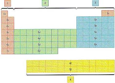
The figure below shows the relationship between the
periodic table and the orbitals being filled during
the aufbau process. The two columns on the left side
of the periodic table correspond to the filling of an s orbital. The
next 10 columns include elements in which the five orbitals
in a d subshell are filled. The six columns on
the right represent the filling of the three orbitals
in a p subshell. Finally, the 14 columns at
the bottom of the table correspond to the filling of the seven orbitals in an f subshell.